UCT Charts

Today’s topic is a little different: it’s as much an art project as it is engineering or science. Pretty graphs below, but first, an introduction.

UCT is messy by computational standards. It wends its way towards perfect play, but the answers you get depend on how long you waited before asking and how fast the hardware was running, not to mention a stream of pseudo-random numbers. An antivirus program running in the background, a network blip on another continent, bubbles in your CPU’s thermal paste – they can all affect what a general game player ends up returning as its move.

So what happens if we take some of that messiness away?

Most of these factors impact the general game player by increasing or decreasing the number of iteration UCT goes through in a game. Suppose we use a single-threaded player and execute an exact number of UCT iterations each turn; then the random numbers become the only factor that change the outcome.

All of a sudden, the choices of moves become probability distributions. And statistics gives us plenty of tools for understanding a distribution by sampling it.

(Technical note: There is still the potential problem of using a random number generator that is sufficiently flawed to skew the results. I took most of the samples in the following charts with Java’s default RNG, which is known to have problems. I’ll be taking future samples with a better source of randomness.)

So here’s a simple question based on that observation: How does the number of iterations of UCT by each player affect the average goal values for a given game? If I double one player’s time to think, how much does that improve their chances of winning?

Statistical theory says that if we get enough samples for each point of interest, we’ll get a decent approximation of that expected value. So we can get a good approximate answer to this question by simply running lots of games under these conditions; and GGP makes this easy to generalize across lots of different games.

Some notes on execution:

All the games shown here are two-player zero-sum games, as these lend themselves perfectly to this type of visualization. The axis on the left is the iteration count of the first player, and the axis on the right is the iteration count of the second player. (I’ve also tried this with some game-theoretic games, but those can only display the goal result of one player and so may be misleading. I’ve omitted them here.)

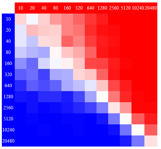
I've been playing around with the color scheme; currently I have a patriotic blue-to-white-to-red, where blue indicates the first player winning, red the second player winning, and white a draw (on average).

These graphs use a logarithmic scale. Each step to the right or down doubles the iteration count. The choice of 10 as a starting point is somewhat arbitrary, but partly it is because the results of UCT are not very interesting when there are fewer iterations than legal moves each turn.

These graphs may also be sensitive to the exact implementations of UCT used. The one used here is a fairly simple version without transposition tables, used in some versions of Alloy 0.10.

Each cell in each graph is the average of at least 93 sample matches.

So let’s take a look:

Tic-Tac-Toe: This is a good chart for seeing how intuition maps to the graph. The first player has a clear advantage, as we would expect; but we can also see the region of playing ability where the players will draw in every match.

Connect Four Suicide: If anything, I had expected the bias to be more obvious; but we can see that it reaches about a 4:1 time handicap by the bottom of the graph.

Connect Four: This game, on the other hand, does appear to give an advantage to the first player at this "skill level", though slighter. (With perfect play, this board size is known to favor the second player.)

Sheep and Wolf: Unfortunately, this doesn’t quite show what I really wanted to show: At some point, the second player should consistently get a forced win, resulting in a huge curve in the results. This graph would make it even more obvious that only the skill of the sheep player, not the wolf player, matters (as pointed out in the game’s Tiltyard statistics). However, this graph mostly just shows the region where the wolf player dominates.

Bidding Tic-Tac-Toe: This is by far the weirdest graph from this set. The second player gets better as expected until around 320-640 iterations, at which point they get worse again. I suspect that this comes down to the second player choosing an appropriate first move of the game in that middle section, then switching to favor a losing first move as its guess of X’s bid changes. (The game is a draw under perfect play by both players.)

As mentioned before, this first move would have a well-defined distribution for any given iteration count, and I could even generate UCT charts conditional on certain starting moves; but I haven’t done this yet.

Dots and Boxes: Of the games I’ve examined so far, this has the “steepest” shift in advantages in the lower right, suggesting that it is the most responsive to increasing iteration counts. It would be nice to know if this continues further down as iteration counts continue to rise.

Dots and Boxes Suicide: By contrast, this variant sees more upset wins; it has no cells in which one player won every game.

You can currently find the full set of generated graphs here: https://alexlandau.github.io/alloybox/abfResultCharts.html

This project has already seen months of computation time on an 8-core machine, and each additional row at the edge of the chart roughly doubles the amount of time needed, so care is needed in many cases to extend this to more games or higher counts. (I had to abandon Speed Chess in particular for being too slow to simulate so many times.)

On a practical level, after working on this project, I’d argue that we should consider using a fixed number of iterations per turn when testing variants of a player against each other. First, it eliminates a number of hardware concerns that could subtly bias results or make them vary from machine to machine. Second, it allows players to be handicapped, to check if a new approach can overcome even an opponent with a computational advantage.

Third, and perhaps most importantly, it helps us test out a new idea – perhaps radically different – and see if it leads to more wins in the games we care about. Often new ideas aren’t as effective as they seem, or require drastic modifications to become useful. Using fixed-iteration tests helps because we can write the new approach with little regard for speed – even console logging can be left in if desired. This way, we can see whether the technique will be effective before we bother to fine-tune it.